Theory of Abstract Interpretation
This note is created for the Cousot POPL77 paper about abstract interpretation^[1] .
Syntax And Semantics of Programs
Syntax
Programs are represented as finite flowcharts, also known as control flow graphs. The graph is built by a set “Nodes”. A node $n \in \text{Nodes}$ is
- An Entry. nodes with no predecessors and one successor
- An Assignment. id(n) := expr(n)
- A Test. A test node has two successors.
forall n in Tests, n-succ(n) = { n-succ-t(n), n-succ-f(n) } - A Junction node has more than 1 predecessor and one successor
- An Exit node has one predecessor and no successor
The set “Arcs” are edges in the graph, that is
Arcs = {<n,m> | (n in Nodes) and (m in n-succ(n))}
Operational Semantics
Let’s define the constructive or operational semantics.
The set “States” are all the information that can occur during computation
States = Arcs^0 times Env
Env = Ident^0 -> Values
Where Values are concrete program values.
So a state in States = <r, e> records that for program point r, the mapping of each variable id to its value.
The initial state is defined as
I-States = {<a-succ(m), bottom | m in Entries >}
i.e. for all entry nodes m, get its successor arc m and set all the variables to empty (bottom, in lattice language).
The state transfer function are defined as equation systems
n-state: States -> States
Its implementation is forward computation. i.e. computing the state of next arc using current arc.
- For test node, the semantics uses
val[test(n)](env)to pick the branch - For assignment node, the semantics uses replacement
env’ = env[val(expr(n))/id(n)]. - …
Finally, a computation sequence is repeatedly apply the state transfer function on the initial state i_s in I-states
s_n = n-state^n(i_s) for n = 0, 1, ...
Consequently, the final state is a the least fixpoint of the functional.
λF.(n-state ∘ F)
i.e. An equation systems is derived by the cfg and the state transfer function, and F in State is a state that no longer change under the equation system :
λF.(n-state ∘ F) (F) = F
Static Semantics
The operational semantics require analysis of every program execution, which is practically impossible for building a realistic verification tool. By Floyd^[2], to prove static properties of program, it is often sufficient to consider the sets of states associated with each program point.
The context is the set of all environments which may be associated in any computation sequences. Context = Pow(Env)
Define the context vector as
Cv: Arcs^0 -> Context
Cv = λq.{e | (exists n >= 0, exists i_s in I-states | <q, e> = n-state^n(i_s))}
Naturally, this represents all the possible program states at program point q. Notice how it is different from the “States” set in operational semantics: it does not care about the execution trace anymore.
It is proved that the context vector is equal to the operational semantics: For all q in Arcs,
- Cv(q) contains at least the environment e which is associated to q during any execution
- Cv(q) contains only the environment e which is associated to q during an execution.
This static view is more suitable for analysis to be performed, which forms the foundation of abstract interpretation: replace sthe concrete Context with abstract context that over-approximates it.
Abstract Interpretation
General Framework
We use A-Cont to as the abstract context which soundly over-approximates the concrete Context.
The set of abstract context vector can be defined as
A-CV = Arcs^0 -> A-Cont
(Note that the paper use \tilde(A-Cont) to represent abstract context but i don’t find it appealing)
We then can find an interpretation that works on the abstract context: `Int: Arcs^0 times A-CV -> A-Cont
Int is supposed to be other-preserving.
Using Int, we can find a system of equations with the program.
Int-CV :: A-CV -> A-CV
Int-CV(CV: A-CV) = λr.Int(r,Cv)
Finally putting everything together, an general abstract interpretation of a program P is a tuple I = <A-Cont, ⊔, ≤, Top, Bottom, Int> where
⊔The join operator on abstract context≤The partial ordering on the abstract context
What is implicit here is that the abstract context is typically designed as a complete lattice, That is, x ≤ y ⇔ x ⊔ y = y. This is a not drastic requirement and proved to be very handy in designing analysis. Typically in ensuring termination and efficient merge contexts by joining.
Example: Data Flow Analysis
Available Expression problem is that asks whether an expression e is available on arc r. Specifically, we want to know if e has been previously computed and since last computation, no argument of the expression has had its value changed.
The abstract context of this problem is a vector that maps all expressions to a boolean value:
B-vect: Expr -> { true, false }
Where Expr is the set of expressions occurring in a program P.
The Int function follows
avail(r, Bv)
  let n be origin(r) within
    case n in
      Entries => λe . false
      Assignments ∪ Tests ∪ Junctions =>
        λe. (generated(n)(e)
             or ( ( ∀ p ∈ a-pred(n). Bv(p)(e) )
                  and transparent(n)(e) ))
    esac
- Nothing is available at the entry nodes.
- An expression
eis available if- e is generated on node
n(ris the exit of noden) - e is available at the predecessors of
nand does not been modified on noden.
- e is generated on node
The analysis is forward reasoning and terminates at the maximal solution of the equation systems generated by avail.
Maximal solution = Starts with every expression to be true.
But more fundamentally: maximality is with respect to the lattice ordering (here:
false ≤ true). So the maximal solution means: among all fixpoints, we take the greatest in that ordering. It’s not just “we want precision”—it’s mathematically required by the chosen ordering.
Why we go for the maximal solution? Considering variables in a loop. if we take the minimal solution, which starts the analysis from all variables to bottom, the variables in the loop might be always “not available”, which is sound but too preservative and not very precise. Rather, the maximum fixpoint is also sound but more precise.
Typology of Abstract Interpretation
There are three dimensions for abstract interpretation according to Cousot:
- Using join (∪) or meet (∩) for junctions
- Forward (→) or backward (←) analysis
- Computing Maximum (↑) or Minimum (↓) fixpoints
Consistent Abstract Interpretation
Let $C_v$ as the concrete context vector and $C_v’$ as the abstract context vector. (A context vector is $Arc \times Cont$)
We can define two functions $\alpha: C_v \to C_v’, \gamma: C_v’ \to C_v$ as the abstraction & concretization function respectively. We typically requires that:
- $\forall x \in \text{A-Cont}, x=\alpha(\gamma(x))$. Concretization losses no information
- $\forall x\in \text{C-Cont}, x \leq \gamma(\alpha(x))$. Allowing abstraction to be only an approximation
In addition, we requires following local hypothesis on the interpretation function: \(\forall(a, x) \in Arcs \times \text{A-Cont}, \gamma(Int(a,x)) \geq Int(a, \gamma(x))\) Which is equivalent to \(\forall(a, x) \in Arcs \times \text{C-Cont}, Int(a, \alpha{(x)}) \geq \alpha(Int(a, x))\) Or, is equivalent to following picture:
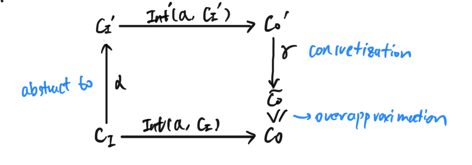
This allows the interpretation to be sound. i.e. The abstract context always over-approximates the concrete one.
The lattice of Abstract Interpretation
For the concrete context of integers. $I_{SS} = Pow(\mathbb{Z})$, we might have abstract interpretations:
- (Intervals $I_I$) $\alpha(S) = [min(a), max(b)]$ Which can be further abstracted as
- (Constant Propagation a $I_{CP}$) $\alpha([a, b]) =$ if $a=b$ then $a$ else $\top$; or
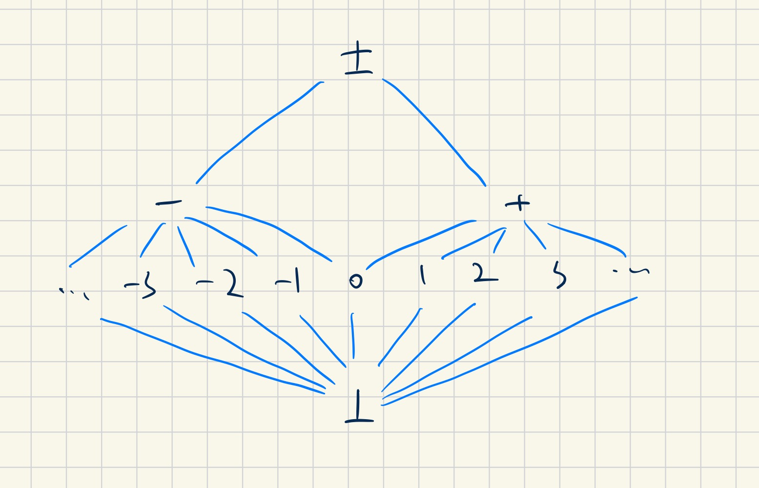
- (Rules of Signs $I_{RS}$) $\alpha([a, b]) =$ if $a \gt 0$ then $+$ elif $b \lt 0$ then $-$ else $\pm$; or
- (Constants + Signs $I_{CS}$) $\alpha([a, b]) =$ if $a = b$ then a elif $a \geq 0$ then $+$ elif $b \leq 0$ then $-$ else $\pm$
- (Reachability $I_R$) $\alpha(i)=$ if $i \neq \bot$ then $\top$ else $\bot$
The context of $I_{CS}$ looks like this:
These interpretation forms a lattice themselves. For example, the interpretations we mentioned can formed a lattice like this:
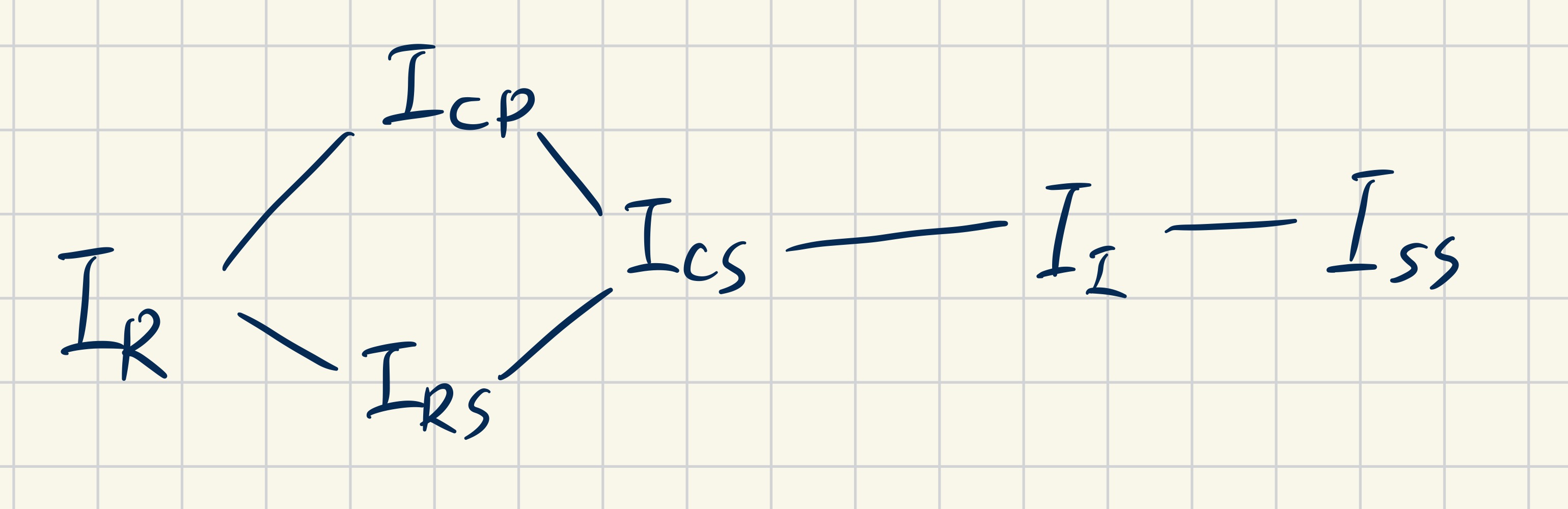 (Actually, $I_R$ is not the bottom as we can find a trivial interpretation that the context lattice is only a single bottom)
If $I_a \gt I_b$, it is generally that $I_a$ is more precise but more computationally expensive. For example, $I_R$ can only detects if a variable is reachable, but would it’s pretty fast on detect unused variables. So the choice of abstraction level really depends on the analysis task.
Abstract Evaluation of Programs
This section briefly mentions the correctness, termination and efficiency proofs of abstract interpretations in related works. If I’m going to do formal correctness proofs then I might go back to this section but now it is interested to me.
Fixpoints Approximation Methods
The sequence of a program’s context is modeled as an ascending Kleen’s sequence: \(Int^n(\bot)\) We typically require $Int$ is designed in such a way this sequence to be not strictly increasing. In particular, through making it order-preserving on the lattice of context. Then an AE terminates when one fixpoint is reached. But this can be slow.
Techniques to approximate the fixpoint can improve. By approximate we mean the AE should satisfies this correctness property: \(\forall n \geq 0,\; C = \widetilde{\text{Int}}^{\,n}(\bot) \;\wedge\; \neg\bigl(\text{Int}(C) \sqsubseteq C \bigr) \;\;\Longrightarrow\;\; C \circ \text{Int}(C) \;\sqsubseteq\; \widetilde{\text{Int}}(C).\) Where $\widetilde{\text{Int}}$ is the approximated interpretation and $\text{Int}$ is the original interpretation. The $\circ$ is the join operator $\sqcup$.
Note: I would argue the condition not (Int(C) <= C) is not necessary. But it is rather used for loosen the condition: it only put requirement on the approximated interpretation when the fixpoint has not been reached. Because after a fixpoint is reached, AE stops naturally.
Widening
Widening is a technique that accelerates the convergence by approximation. A widening $\nabla: ACont \times ACont \to ACont$ is a binary operator such that
- $\forall (C, C’) \in ACont^2, C \nabla C’ \ge C \sqcup C’$
- With arbitrary sequence $C_i$ of $ACont$, The sequence is not strictly increasing: $x_{0}, \quad x_{1} = x_0 \nabla C_0, \quad x_{2} = x_1 \nabla C_1, \quad \dots$
The first one ensures widening “goes up” on the lattice. I found it more intuitive to explain why is that going “up” in the context lattice always safely over-approximates the concrete context but goes “down” might lose soundness.
The second one is also for termination of course.
We also labels the arc which has been performed widening by adding them into the $\text{W-Arcs}$ set.
Finally, the approximated interpretation is:
A-Int q, Cv = if q in W-Arcs then
  Cv(q) ∇ Int(q, Cv)
else
  Int(q, Cv)
fi
They proved that the correctness property (at the beginning of this section) is satisfied.
Note that the two requirements of widening does not limit how precise the operator ∇ is designed. An extreme but valid one is simply ∇ _ _ = top, but this will produce very imprecise over-approximation. So also we try to be as precise as possible.
Narrowing
Widening produces an upper bound $S_m = \widetilde{\text{A-Int}}^m(\bot)$ of the least fixpoint of the (un-approximated) interpretation $C_v = \widetilde{\text{Int}}^n(\bot)$. i.e. $S_m \ge C_v$. If $S_m$ is not a fixpoint of $\text{Int}$, we might want to find a better approximation $C_v \leq S’_m \leq S_m$. (For notation: $\widetilde{\text{Int}}$ is the whole program interpretation and $\widetilde{\text{A-Int}}$ is modified from $\widetilde{\text{Int}}$ by adding widening)
A binary operator △: A-Cont × A-Cont → A-Cont is a narrowing if it satisfies two requirements:
∀ (C, C') ⋿ A-Cont ⨉ A-Cont, { C ≥ C} → { C ≥ C △ C' ≥ C' }- For any arbitrary sequence
C0, C1, ... Cn, ..., the infinite sequenceS(0) = C0, S(n) = S(n-1) △ Cnis not strictly decreasing.
And we can modify the interpretation as:
D-Int q Cv =
	if q in W-arcs then
		Cv(q) △ Int(q, Cv)
	else
		Int(q, Cv)
	fi
Mathematical Intuition of Narrowing
The second requirement of narrowing is straightforward: we want to ensure termination of the D-Int function. But the first one is a bit random at the first glance. I want to take a note here to explain it.
Remember $S_m$ is produced by the approximated interpretation ($\widetilde{\text{Int}}$ with widening), then $S_m$ is no less than $C_v$, the least fixpoint of $\widetilde{\text{Int}}$. We have $\widetilde{\text{Int}}(S_m) \leq S_m$ since $\widetilde{\text{Int}}$ is required to be order-preserving. And therefore we can construct a descending sequence: \(\text{DKS}: S_m \ge \widetilde{\text{Int}}(S_m) \ge \widetilde{\text{Int}}^2(S_m) \ge \dots \ge \widetilde{\text{Int}}^n(S_m) \ge C_v\) So the limit of $\widetilde{\text{Int}^i}(S_m), \forall i \in \mathbb{N}$ is sure a better approximation of $C_v$. A naive approach is to repeatedly applying $\widetilde{\text{Int}}$. But we face a same problem as widening: DKS can be computationally expensive to converge; Or it might be an infinite sequence. So it is practical to soundly truncate the sequence.
From step n, the most ideal truncate point D might satisfies
\(\widetilde{\text{Int}}^{n+1}(S_m) \gt D \ge C_v \tag{CoT'}\)
However, we do not know $C_v$ in the practice. Hence this condition gives little information about how to choose a $D$.
So we have to modify the correctness of truncate as
\(\widetilde{\text{Int}}^{n+1}(S_m) \gt D \ge \widetilde{\text{Int}}(D) \tag{CoT}\)
It is sound to replace $C_v$ because it is the least fixpoint and interpretation is order-preserving.
This is where the first condition comes from: The D-Int satisfies CoT by case analysis: when q ⋿ W-arcs, applying the first requirement get us CoT; otherwise, CoT trivially holds because interpretation is order-preserving.
References
^[1]: Cousot, Patrick, and Radhia Cousot. “Abstract Interpretation: A Unified Lattice Model for Static Analysis of Programs by Construction or Approximation of Fixpoints.” Proceedings of the 4th ACM SIGACT-SIGPLAN Symposium on Principles of Programming Languages - POPL ’77, ACM Press, 1977, 238–52. https://doi.org/10.1145/512950.512973
^[2]: Floyd, Robert W. “Assigning meanings to programs.” Program Verification: Fundamental Issues in Computer Science. Dordrecht: Springer Netherlands, 1993. 65-81.